Graph Neural Networks
Graph Neural Networks
1. Basic Concepts
2. Centrality
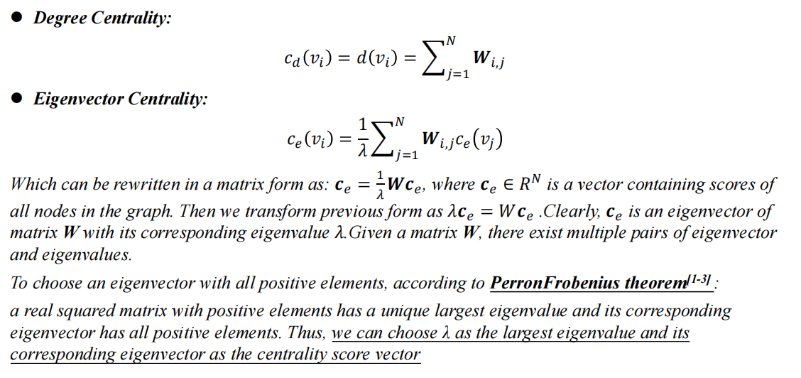
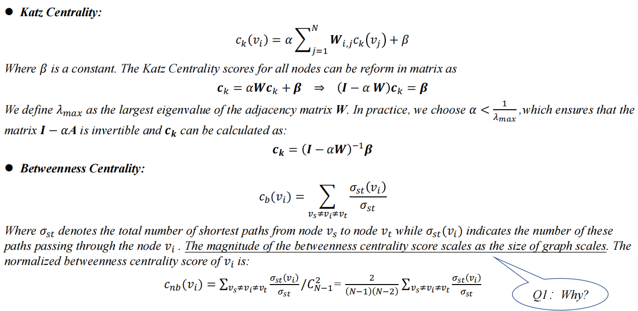
The centrality of a node measures the importance of the node in the graph
the bigger the $c_b(v_i)$ is, the more importance node i is: without node i most shortest ways would disappear.
3. Spectral Graph Theory
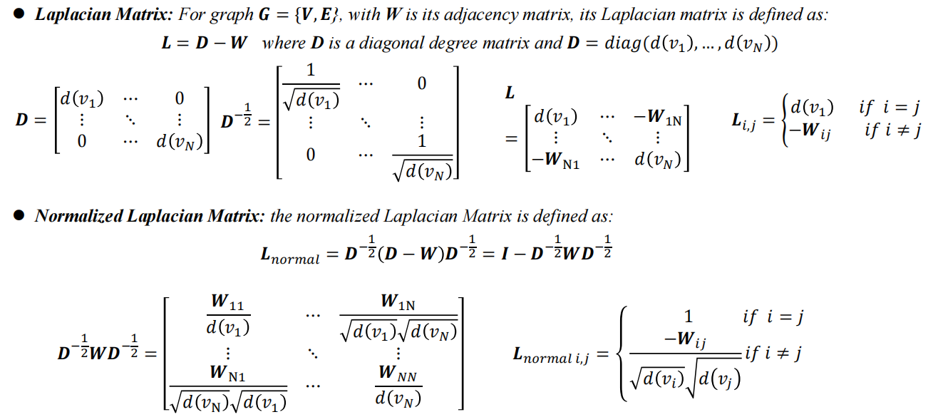
Why we want to normalize the Laplacian Matrix?
In my opinion, take $W_{ij}$ as an example, maybe $d(v_i)$ or $d(v_j)$ is very big, so that the $W_{ij}=1$ may not be as important as the connecting nodes with small degrees.
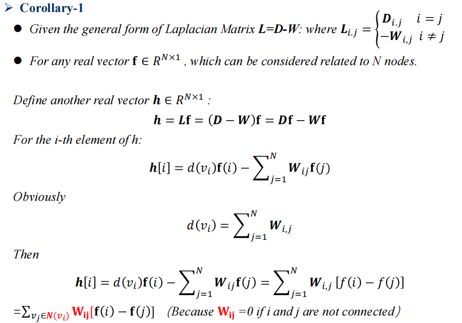
Corollary 1
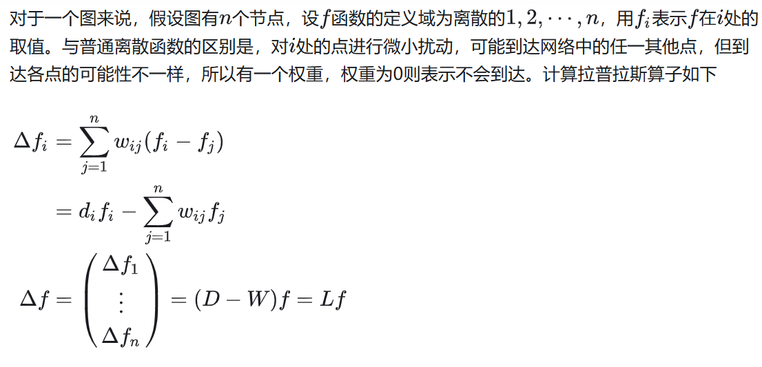
It much easy to comprehend how people come up with $L$ like this — We want to describe the variation between discrete $f$ 图傅里叶变换 - 知乎
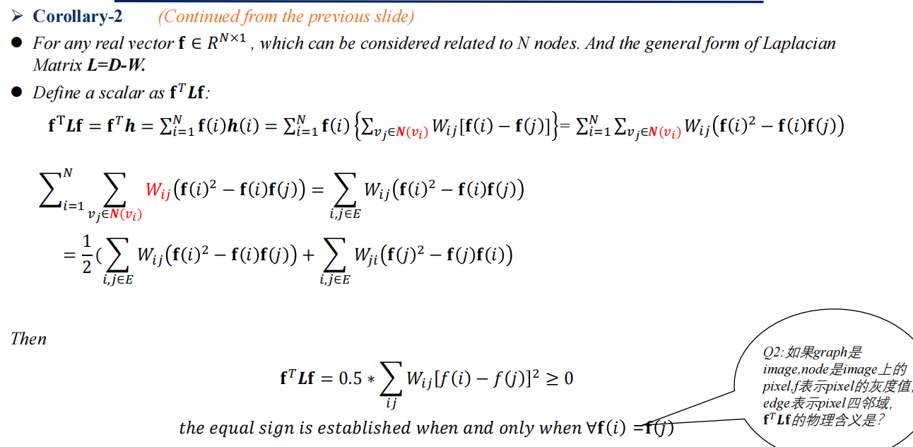
Corollary 2
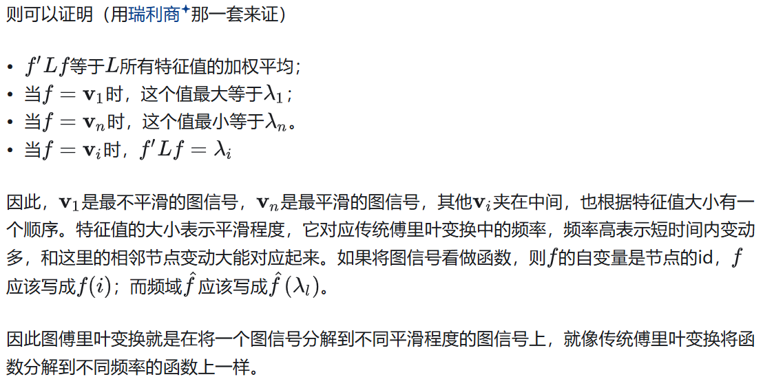
$f^TLf$ can represent the smoothness of signal $f$.
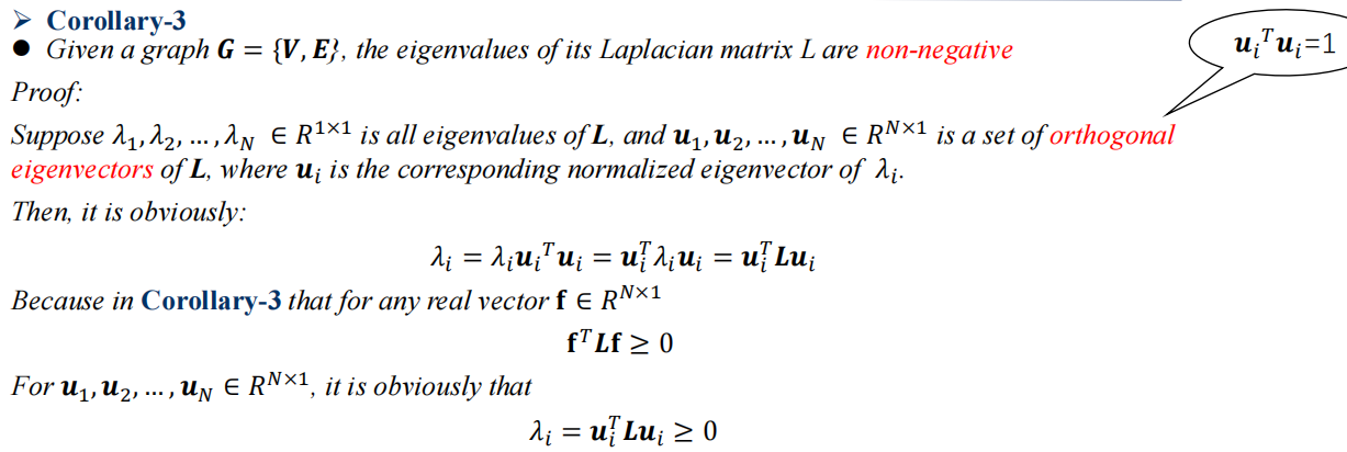
Corollary 3
Initially, $f$ can be any vector, in corollary 3 we change it into orthogonal eigenvectors of $L$ — $u$ .
Corollary 4
4. Graph Partition
Graph Classifications
Note 1
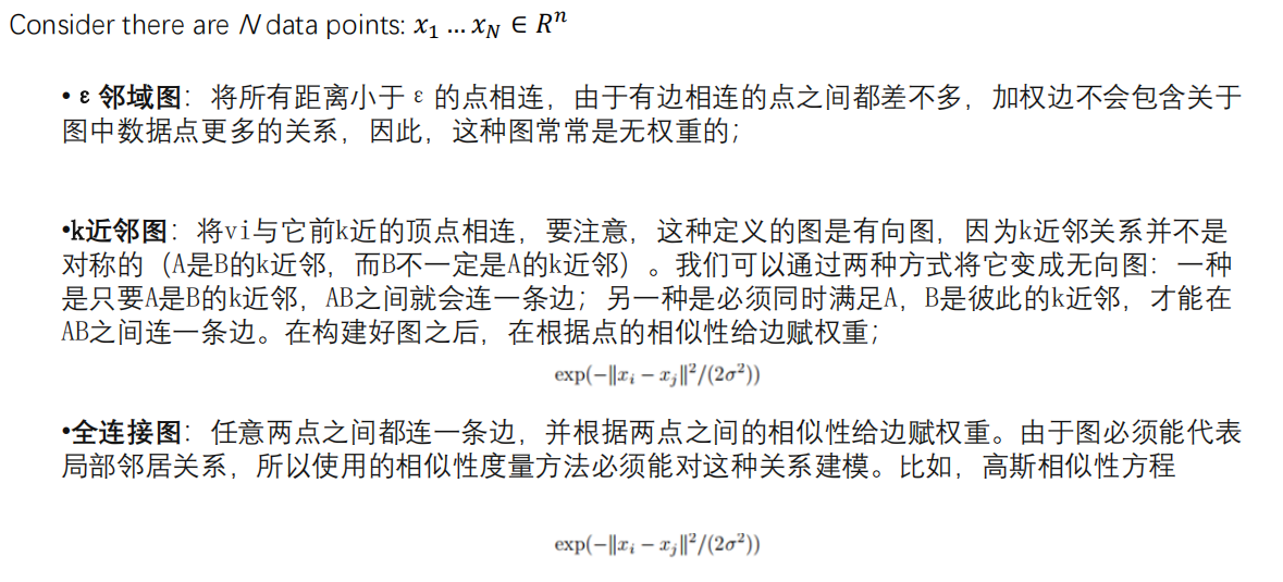
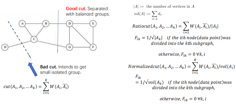
- Data clustering was modeled as graph partition.
- Similar data points are connected by links. Weight intensity implies their similarities.
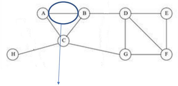
- When dividing the graph, we intends to ‘cut’ the weakest links connecting two subgraphs.
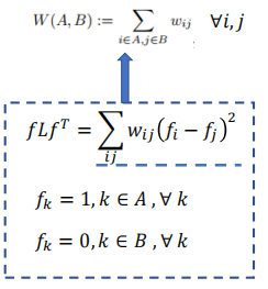
The equation above illustrates how to find the weakest edge to “cut”, which means that when this edge disappears, the least connection in this graph would be damaged or influenced.
Note 2
Since that the method above is so silly, we want to find an exquisite way which is fitter for computer calculation.
Alternative settings:
What we need is just $ f_A-f_B =1$ We input all the possibilities of vector $f$ , the one with the smallest output $fLf^T$ is the best graph partition.
Multiple graph partition
For a given number $k$ of subsets/subgraphs, the mincut approach simply choose a partition $A_1,A_2,A_3,…,A_k$ , which minimize :
\[cut(A_1,A_2,...,A_k)=\frac{1}{2}\sum_{i=1}^k{W\left( A_i,\overline{A_i} \right)}\]We design the indicator matrix,
\[F\in R^{N\times K}\] \[\left[ \begin{matrix} f_{1}^{T}Lf_1& & & \\ & f_{2}^{T}Lf_2& & \\ & & ...& \\ & & & f_{k}^{T}Lf_k\\ \end{matrix} \right] \,\,\] \[cut(A_1,A_2,...,A_k):=min (trace(F^TLF))\]Normalized cut
5. Spectral Clustering
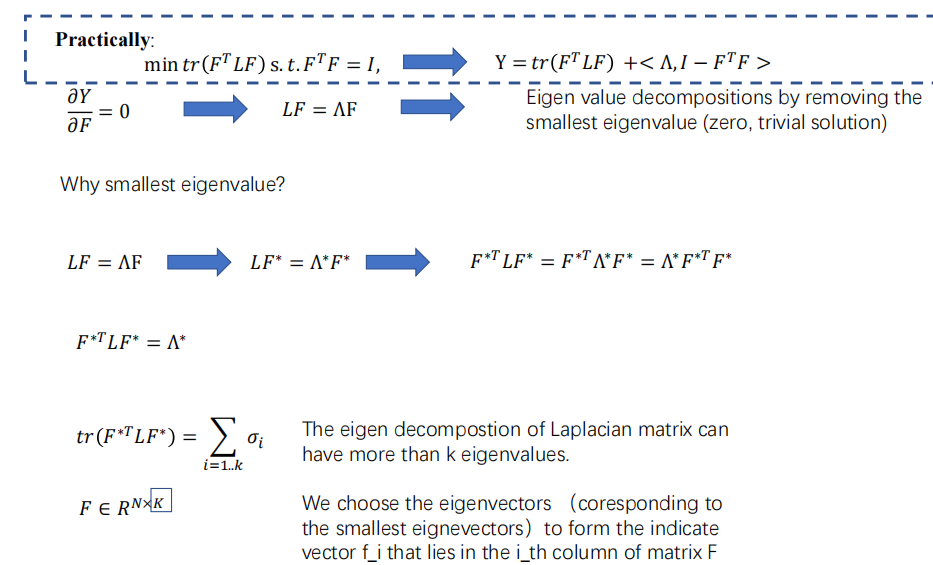
By the way, the input $F$ should satisfy: (also, we normalize it before)
\[F^TF=I\]because of non-overlaps of subgraphs (They should not contain each other’s nodes)
Actually, We select the eigenvectors of the top 7 smallest eigenvalues (removing zero,trivial solution)
6. Graph Fourier Transform
Graph Signal Process
A graph is smooth if the values in connected nodes are similar. A smooth graph signal is with low frequency, as the values change slowly across the graph via the edges.
The value $f^TLf$ is called as the smoothness ( or the frequency ) of the signal $f$.
Graph Fourier Transform
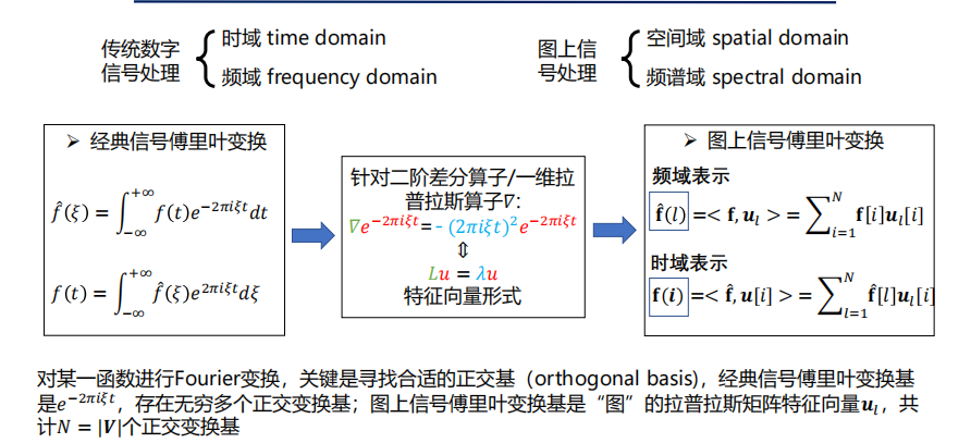
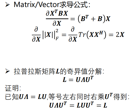
对图信号进行傅里叶变换:用拉普拉斯矩阵的特征向量作为图傅里叶投影的基。设拉普拉斯矩阵可进行如下特征分解: \(L=U\varLambda U^T\)
其中U的每一列都是L的特征向量,$\varLambda$ 是个对角矩阵,对角元是L的特征值。这里考虑无向图,$L$ 是对称矩阵,一定可以进行这样的特征分解。则图傅里叶变换定义为:
\[\hat{f}=U^T f\]图傅里叶逆变换如下:
\[f=U\hat{f}=UU^T f=f\]7. Common GNN Structures
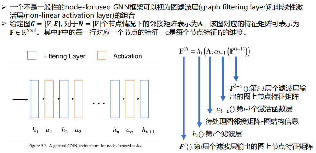
node-focused
任务的目标是学习节点层面的特征
- 图滤波层
- 非线性激活层
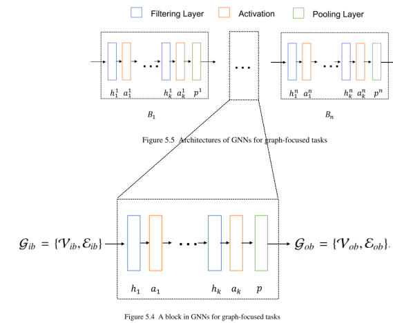
graph-focused
目标是学习整个图的代表性特征,而学习节点特征通常是一个中间步骤,而学习节点特征的过程通常同时利用输入节点特征和图结构
- 图滤波层
- 非线性激活层
- 图池化层
Graph filter
Spectral Filtering
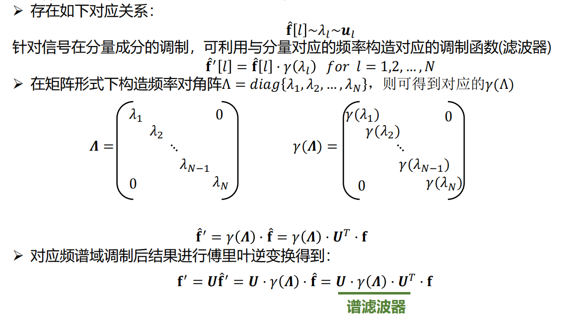
核心思路:
是在频谱域,对图上信号各个频率(频谱)成分对应的系数进行调制,使得部分有用的频率成分被保留/放大,部分无用的频率成分被移除/衰减。
相当于先变到频域空间,再对每一个维度进行调制,然后再变回去
Regularization Term
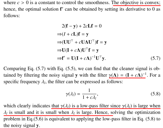
\[\mathop {arg\min} \limits_{f}\left\| f-y \right\| ^2+cf^TLf\]Suppose that we are given a noisy graph signal $y=f_0+\eta$ defined on a graph $\boldsymbol{G}$ ,where $\eta$ is uncorrelated additive Gaussian noise, we wish to recover the original signal $f_0$ .
To enforce the prior information of the smoothness of the clean signal $f_0$, we introduce the regularization term above.
A low-pass filter
Polynomial Filter Operator (多项式滤波器)
Handle multi-channel information(处理多通道信息)
单通道输出
单通道输出的定义是:
\[f_{\text{out}} = \sum_{d=1}^{d_{\text{in}}} U \cdot \gamma_d(\Lambda) \cdot U^T \cdot F_{:,d}\]这里,输入特征 $F_d $ 是一个 $d_{\text{in}} $ 维信号,每一维输入信号经过特定的滤波器 $\gamma_d(\Lambda) $进行卷积操作后再求和,最终生成一个单通道输出。
其实,可以将 $ U \cdot \gamma_d(\Lambda) \cdot U^T $ 看做一个谱滤波器,也类似于卷积操作,对每一个输入信号 $F_{:,d}$ 进行滤波处理,然后将得到的结果全部求和输出一个结果。
多通道输出
在多通道输出中,公式是:
\[F_{:,j} = \sum_{d=1}^{d_{\text{in}}} U \cdot \gamma_{j,d}(\Lambda) \cdot U^T \cdot F_{:,d}\]其中 $j=1,2,…,d_{\text{out}} $。
这里,每个输出通道 $j$ 有自己的一组滤波器 $\gamma_{j,d}(\Lambda) $,这些滤波器分别作用于每个输入通道,然后通过求和得到第 $j $ 个输出通道。通过不同的滤波器参数,最终可以生成 $ d_{\text{out}} $ 个输出通道。
其实本质上和单通道输出一样,只是现在有和输出通道数一样多的不同$ U \cdot \gamma_d(\Lambda) \cdot U^T $ 滤波器,需要将原来的过程重复 $d_{out}$ 次即可。
多通道GCN输出
通常,一个简单的GCN-Filter核函数应该是:
\[f^{\prime}=\theta \tilde{D}^{-\frac{1}{2}}\tilde{A}\tilde{D}^{-\frac{1}{2}}f\]我们就定义 $K=\tilde{D}^{-\frac{1}{2}}\tilde{A}\tilde{D}^{-\frac{1}{2}}\in R^{N\times N}$ 为“卷积核”,和卷积神经网网络中的卷积核效果一致,其中不同的参数 $\theta$ 表示不同的卷积核参数。
总体也和上部分的多通道输出没有本质区别,只是选取了不同的滤波函数而已。
\[F_{:,j} = \sum_{d=1}^{d_{\text{in}}}\theta_{j,d} K F_{:,d}\]其中 $j=1,2,…,d_{\text{out}} $,$F^{\prime}=KF\varTheta ,where\,\,\varTheta \in R^{d_{in}\times d_{out}}$
